Demo Script
Identity intensity function
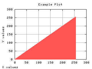
The simplest intensity function is the identify s=v. This transform is a line of 45 degrees. It makes the output image the same as the input image.


Visualizing the intensity transform function

Changing a particular color of an image
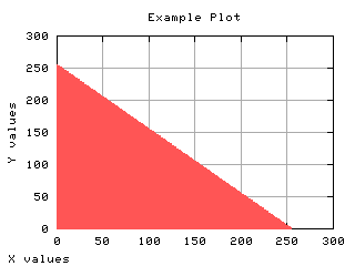
To change a given gray scale value v1 of the input image to another gray scale value s1, we can change the identity function such that T(v1)=s1. Suppose we want to change any pixel with value 0 to 255.
>>> it1 = 1*it
>>> it1[0] = 255
>>> print it1[0:5] # show the start of the intensity table
[255 1 2 3 4]
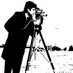
>>> g = iaapplylut(f, it1)
>>> iashow(g)
(100, 100) Min= 28 Max= 255 Mean=152.700 Std=77.37
 |
|
| g |
Negative of an image
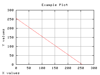
To invert the gray scale of an image, we can apply an intensity transform of the form T(v) = 255 - v. This transform will make dark pixels light and light pixels dark.
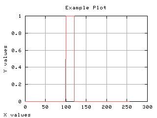
Thresholding
A common operation in image processing is called thresholding. It assigns value 1 to all pixels equal or above a threshold value and assigns zero to the others. The threshold operator converts a gray scale image into a binary image. It can be easily implemented using the intensity transform. In the example below the threshold value is 128.
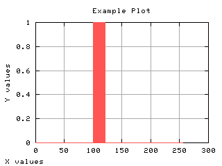
Threshold band
A variation of the thresholding is when the output is one for a range of the input gray scale values. In the example below, only pixels between values 100 and 120 are turned to one, the others to zero.
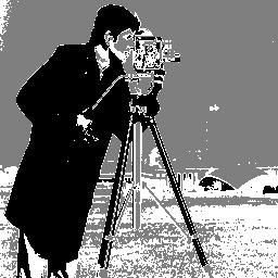
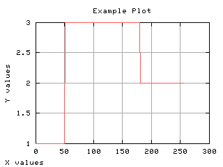
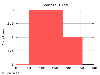
Generalized Threshold
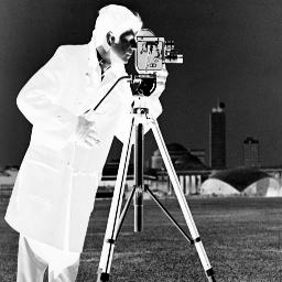
A generalization of the previous case is to assign different values (classes) to different input ranges. This is a typical classification decision. For pixels from 0 and t1, assign 1; from t1 to t2, assign 2, etc. In the example below, the pixels are classified in three categories: class 1: dark pixels (between 0 and 50) corresponding to the cameraman clothing, class 3: medium gray pixels (from 51 to 180), and class 2: white pixels (from 181 to 255), corresponding to the sky.
Crescent functions
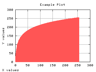
When the intensity transform is a crescent function, if v1 >= v1 then T(v1) >= T(v2). In this class of intensity transforms, the order of the gray scale does not change, i.e., if a gray scale value is darker than another in the input image, in the transformed image, it will still be darker. The intensity order does not change. This particular intensity transforms are of special interest to image enhancing as our visual system does not feel confortable to non-crescent intensity transforms. Note the negation and the generalized threshold examples. The identity transform is a crescent function with slope 1. If the slope is higher than 1, for a small variation of v, there will be a larger variation in T(v), increasing the contrast around the gray scale v. If the slope is less than 1, the effect is opposite, the constrast around v will be decreased. A logarithm function has a higher slope at its beginning and lower slope at its end. It is normally used to increase the contrast of dark areas of the image.
>>> v = Numeric.arange(256)
>>> Tlog = (256./Numeric.log(256.)) * Numeric.log(v + 1)
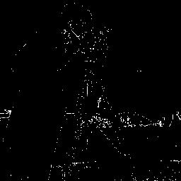
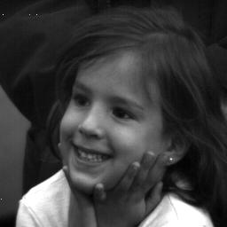
>>> f = ianormalize(iaread('lenina.pgm'), [0, 255])
>>> g = iaapplylut(f.astype('b'), Tlog)
>>> iashow(f)
(256, 256) Min= 0 Max= 255 Mean=61.170 Std=54.05
>>> iashow(g)
(256, 256) Min= 0.0 Max= 256.0 Mean=177.107 Std=34.66
>>> g,d = iaplot(Tlog)
>>> g('set data style boxes')
>>> g.plot(d)
>>>
 |
 |
|
| f | g |
 |
 |
|
| Tlog | d |