iahotelling

Image creation

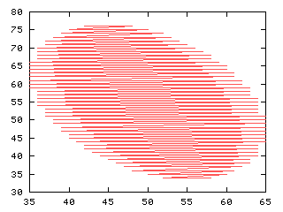
A binary image with an ellipsis

>>> f = iagaussian([100,100], [45,50], [[20,5],[5,10]]) > 0.0000001

>>> iashow(f)

(100, 100) Min= 0 Max= 1 Mean=0.098 Std=0.30


f

Feature vector

The coordinates of each 1 pixel are the features: cols and rows coordinates. The mean value is the centroid.

>>> import Numeric, MLab

>>> (rows, cols) = iaind2sub(f.shape, Numeric.nonzero(Numeric.ravel(f)))

>>> x = Numeric.concatenate((cols[:,Numeric.NewAxis], rows[:,Numeric.NewAxis]), 1)

>>> mx = MLab.mean(x)

>>> print mx

[ 50.  45.]

Computing eigenvalues and eigenvectors

The eigenvalues and eigenvectors are computed from the covariance. The eigenvalues are sorted in decrescent order

>>> Cx = MLab.cov(x)

>>> print Cx

[[  59.31288344   29.65644172]
 [  29.65644172  117.32924335]]

>>> [aval, avec] = MLab.eig(Cx)

>>> aux = Numeric.argsort(aval)[::-1]

>>> aval = MLab.diag(Numeric.take(aval, aux))

>>> print aval

[[ 129.8057478     0.        ]
 [   0.           46.83637899]]

>>> avec = Numeric.take(avec, aux)

>>> print avec

[[-0.38778193 -0.92175115]
 [-0.92175115  0.38778193]]

Measure the angle of inclination

The direction of the eigenvector of the largest eigenvalue gives the inclination of the elongated figure

>>> a1 = Numeric.sqrt(aval[0,0])

>>> a2 = Numeric.sqrt(aval[1,1])

>>> vec1 = avec[:,0]

>>> vec2 = avec[:,1]

>>> theta = Numeric.arctan(1.*vec1[1]/vec1[0])*180/Numeric.pi

>>> print 'angle is %3f degrees' % (theta)

angle is 67.183445 degrees

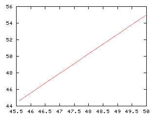
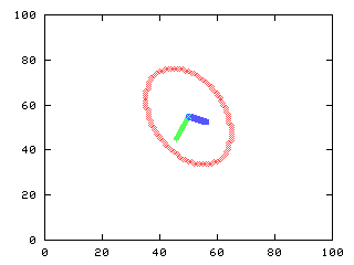
Plot the eigenvectors and centroid

The eigenvectors are placed at the centroid and scaled by the square root of its correspondent eigenvalue

>>> iashow(f)

(100, 100) Min= 0 Max= 1 Mean=0.098 Std=0.30

>>> x_,y_ = iaind2sub(f.shape, Numeric.nonzero(Numeric.ravel(iacontour(f))))

>>> g,d0 = iaplot(y_, 100-x_)

>>> # esboça os autovetores na imagem

>>> x1, y1 = Numeric.arange(mx[0], 100-mx[0]+a1*vec1[0], -0.1), Numeric.arange(mx[1], mx[1]-a1*vec1[1],0.235)

>>> g,d1 = iaplot(x1, 100-y1) # largest in green

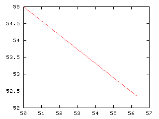
>>> x2, y2 = Numeric.arange(mx[0], mx[0]-a2*vec2[0], 0.1), Numeric.arange(mx[1], mx[1]+a2*vec2[1],0.042)

>>> g,d2 = iaplot(x2, 100-y2) # smaller in blue

>>> g,d3 = iaplot(mx[0], 100-mx[1]) # centroid in magenta

>>> g('set data style points')

>>> g('set xrange [0:100]')

>>> g('set yrange [0:100]')

>>> g.plot(d0, d1, d2, d3)

>>>


f	y_, 100-x_


x1, 100-y1	x2, 100-y2


mx[0], 100-mx[1]	d0, d1, d2, d3

Compute the Hotelling transform

The Hotelling transform, also called Karhunen-Loeve (K-L) transform, or the method of principal components, is computed below

>>> y = Numeric.transpose(Numeric.matrixmultiply(avec, Numeric.transpose(x-mx)))

>>> my = MLab.mean(y)

>>> print my

[ 8.34651835e-017 -2.23178643e-016]

>>> Cy = MLab.cov(y)

>>> print Cy

[[ 1.29805748e+002 -5.53976315e-015]
 [-5.53976315e-015  4.68363790e+001]]

>>> print Numeric.floor(0.5 + Numeric.sqrt(Cy))

math domain error

Display the transformed data

The centroid of the transformed data is zero (0,0). To visualize it as an image, the features are translated by the centroid of the original data, so that only the rotation effect of the Hotelling transform is visualized.

>>> ytrans = Numeric.floor(0.5 + y + Numeric.resize(mx, (x.shape[0], 2)))

>>> g = Numeric.zeros(f.shape)

>>> i = iasub2ind(f.shape, ytrans[:,1], ytrans[:,0])

>>> Numeric.put(g, i, 1)

>>> iashow(g)

(100, 100) Min= 0 Max= 1 Mean=0.094 Std=0.29


g

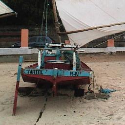
Image read and display

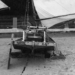
The RGB color image is read and displayed

>>> f = iaread('boat.ppm')

>>> iashow(f)

(3, 257, 256) Min= 0 Max= 218 Mean=94.533 Std=57.35


f

Extracting and display RGB components

The color components are stored in the third dimension of the image array

>>> r = f[0,:,:]

>>> g = f[1,:,:]

>>> b = f[2,:,:]

>>> iashow(r)

(257, 256) Min= 0 Max= 218 Mean=101.268 Std=59.14

>>> iashow(g)

(257, 256) Min= 0 Max= 211 Mean=94.919 Std=56.92

>>> iashow(b)

(257, 256) Min= 0 Max= 201 Mean=87.413 Std=55.07


r	g


b

Feature vector: R, G and B values

The features are the red, green and blue components. The mean vector is the average color in the image. The eigenvalues and eigenvectors are computed. The dimension of the covariance matrix is 3x3 as there are 3 features in use

>>> x = 1.*Numeric.concatenate((Numeric.ravel(r)[:,Numeric.NewAxis], Numeric.ravel(g)[:,Numeric.NewAxis], Numeric.ravel(b)[:,Numeric.NewAxis]), 1)

>>> mx = MLab.mean(x)

>>> print mx

[ 101.26770732   94.9191999    87.41316573]

>>> Cx = MLab.cov(x)

>>> print Cx

[[ 3497.95108557  3273.20413327  3086.73663437]
 [ 3273.20413327  3239.67139072  3103.11181452]
 [ 3086.73663437  3103.11181452  3032.39588874]]

>>> [aval, avec] = MLab.eig(Cx)

>>> aux = Numeric.argsort(aval)[::-1]

>>> aval = MLab.diag(Numeric.take(aval, aux))

>>> print aval

[[ 9572.66965395     0.             0.        ]
 [    0.           180.2290775      0.        ]
 [    0.             0.            17.11963358]]

>>> avec = Numeric.take(avec, aux)

>>> print avec

[[-0.59515464 -0.58010086 -0.55612404]
 [-0.76785348  0.20637147  0.60647494]
 [ 0.2370485  -0.78796815  0.5682554 ]]

Hotelling transform

The K-L transform is computed. The mean vector is zero and the covariance matrix is decorrelated. We can see the values of the standard deviation of the first, second and third components

>>> y = Numeric.transpose(Numeric.matrixmultiply(avec, Numeric.transpose(x-mx)))

>>> my = MLab.mean(y)

>>> print my

[ 1.86724609e-013  9.30065579e-015  1.03426779e-014]

>>> Cy = MLab.cov(y)

>>> print Cy

[[ 9.57266965e+003 -8.78852081e-011 -7.44802346e-011]
 [-8.78852081e-011  1.80229077e+002 -7.44824028e-012]
 [-7.44802346e-011 -7.44824028e-012  1.71196336e+001]]

>>> Cy = Cy * (1 - (-1e-10 < Cy < 1e-10))

>>> print Numeric.floor(0.5 + Numeric.sqrt(Cy))

[[ 98.   0.   0.]
 [  0.  13.   0.]
 [  0.   0.   4.]]

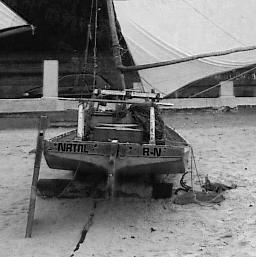
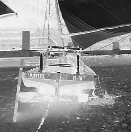
Displaying each component of the transformed image

The transformed features are put back in three different images with the g1 with the first component (larger variance) and g3 with the smaller variance

>>> g1 = y[:,0]

>>> g2 = y[:,1]

>>> g3 = y[:,2]

>>> g1 = Numeric.reshape(g1, r.shape)

>>> g2 = Numeric.reshape(g2, r.shape)

>>> g3 = Numeric.reshape(g3, r.shape)

>>> iashow(g1)

(257, 256) Min= -194.702376045 Max= 163.945218189 Mean=0.000 Std=97.84

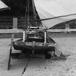
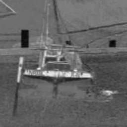
>>> iashow(g2)

(257, 256) Min= -53.4192670921 Max= 81.6627408632 Mean=0.000 Std=13.42

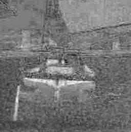
>>> iashow(g3)

(257, 256) Min= -17.361967919 Max= 20.538452635 Mean=0.000 Std=4.14


g1	g2


g3

iahotelling
Illustrate the Hotelling Transform

Demo Script

Image creation

Feature vector

Computing eigenvalues and eigenvectors

Measure the angle of inclination

Plot the eigenvectors and centroid

Compute the Hotelling transform

Display the transformed data

Image read and display

Extracting and display RGB components

Feature vector: R, G and B values

Hotelling transform

Displaying each component of the transformed image

iahotelling Illustrate the Hotelling Transform

Demo Script

Image creation

Feature vector

Computing eigenvalues and eigenvectors

Measure the angle of inclination

Plot the eigenvectors and centroid

Compute the Hotelling transform

Display the transformed data

Image read and display

Extracting and display RGB components

Feature vector: R, G and B values

Hotelling transform

Displaying each component of the transformed image

iahotelling
Illustrate the Hotelling Transform