 |
 |
|
|
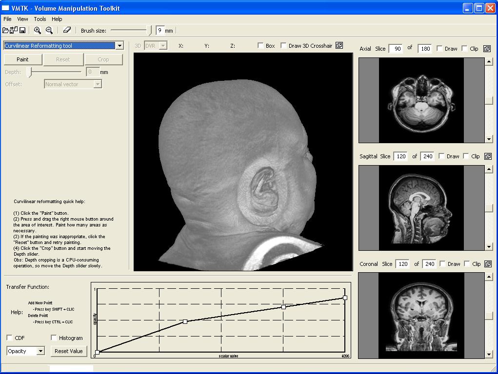 |
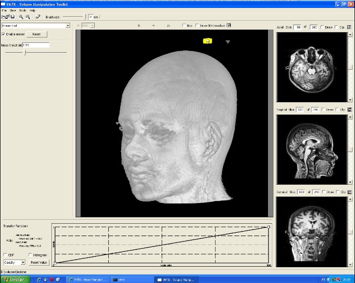
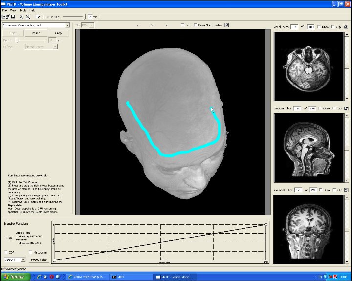
This image illustrates the user interface of our prototype. It consists of a top toolbar from which menus may be enabled, canvas and panels. The center canvas shows the 3D-rendition of the loaded 3D MRI image, while the three smaller canvas on the right side present the coronal, sagittal, and transverse planes of the brain. The left side is the panel for parameter setting of each operation mode. There are three operation modes: 3D erasing, curvilinear reformatting, and measuring. In this image the current mode is the curvilinear reformatting one. The transfer function editor lies in the lower left corner. Observe that the volume sizes are shown on the top of each 2D view canvas. | 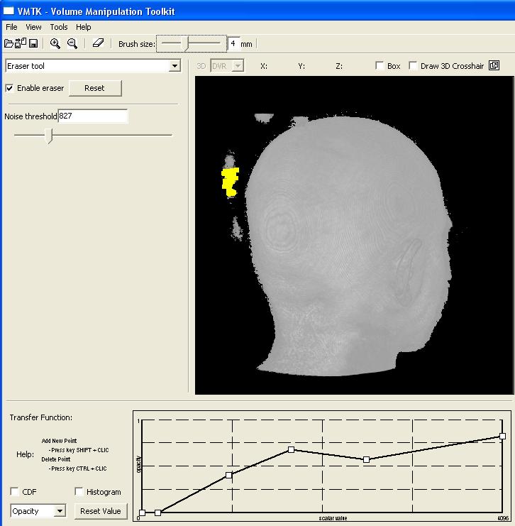 |
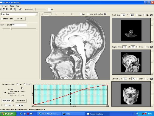
This image shows the control panel for 3D erasing. Through this panel the user can set the scalar value to be considered as the one of the scalp (Noise threshold). All values less than this threshold are ignored until the scalp. In this image, the chosen threshold is 827. To remove locally the noises, a "brush tool" may be used. The brush size is adjustable by the slider on the bar below the top tool bar. In this picture it is set at 4mm. The visual feedback is provided by a yellow shade at the tip of the cursor and all the visible noises in the painted region are removed. In the current version, if there are more than one noise sample along the picking ray, the user needs to pass the cursor over the region several times to remove them completely (see the video). |
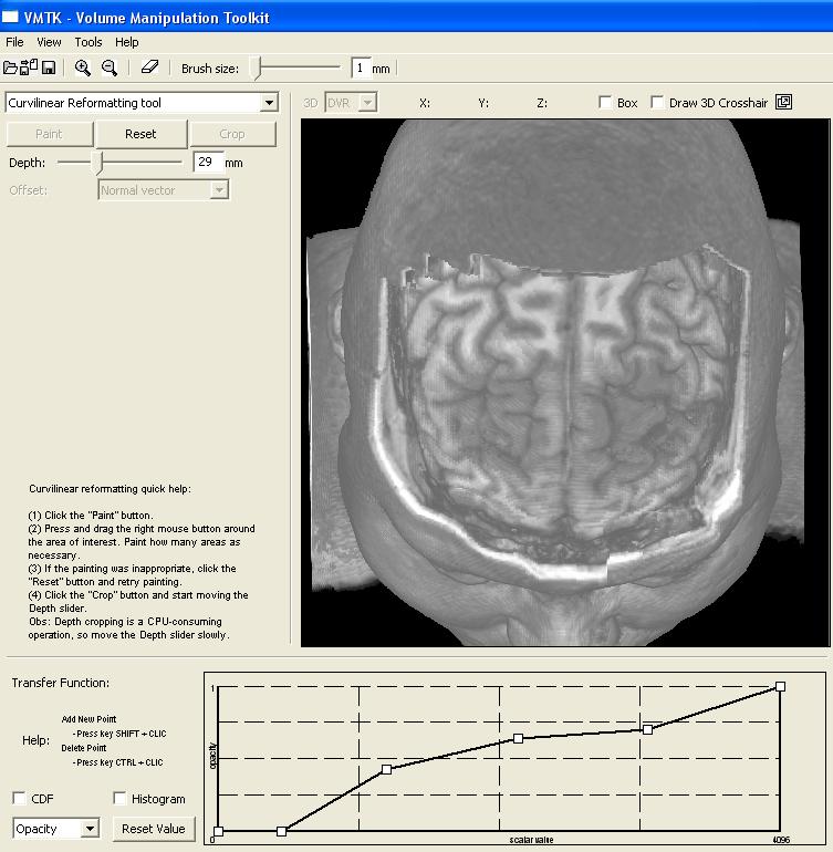 |
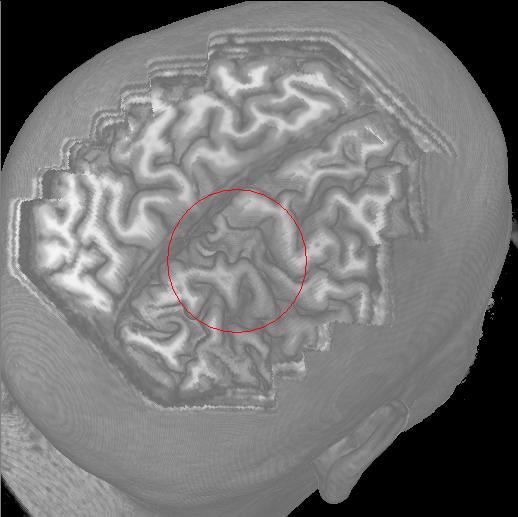
This image depicts the control panel for curvilinear reformatting. First, the user should select the region of interest by painting on the scalp. Second, the button "Crop" should be pressed to perform cropping in a fixed depth. Then, through the depth slider the user may visualize the intermediary slices. In this image the cropping depth is 27mm. "Reset" button may be applied to re-initialize the control volume and the original volume data is restored (see the video). |
| In our prototype the user controls separately the transfer function from the image scalar values to the grayscale values and to the opacity. This pictures shows the transfer function of the grayscale values while the image presents the transfer function of the opacity. Both transfer functions are employed in the volume rendering. The user may design her/his own transfer function by inserting or deleting the control points in the graphs. In this case, five and three control points have been inserted in the opacity and grayscale transfer functions, respectively (see the video). | |
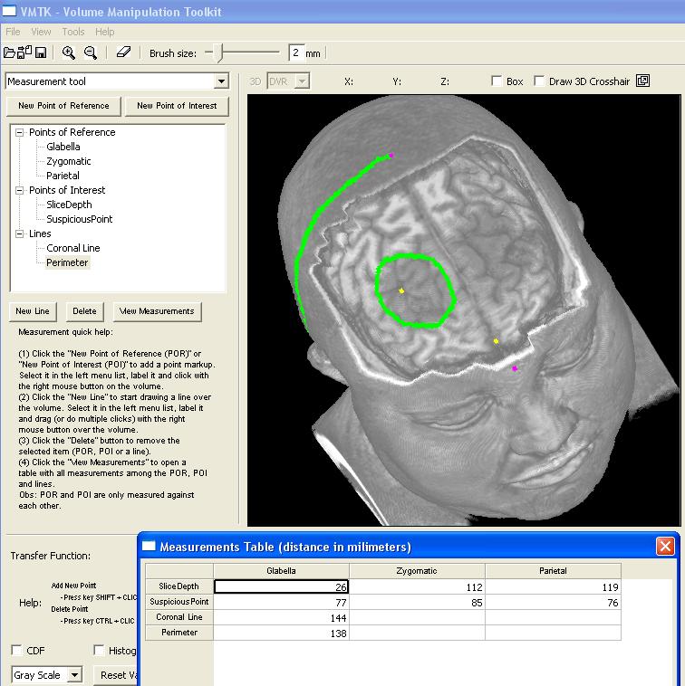 |
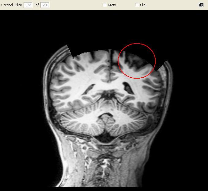
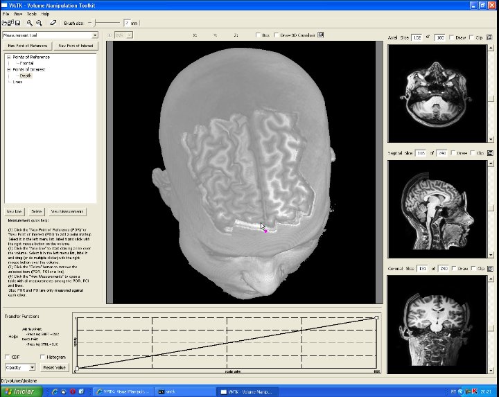
This image highlights the control panel for measuring. Three classes of elements are distingushed: points of reference (magenta), points of interest (yellow) and lines (green). Whnever a new element is defined, the user should name it in the TreeControl widget. Automatically, the distance between each pair (point of reference, point of interest) and the length of lines are computed. These measures can be read from the measurement table that is popped up when the user clicks on the "View Measurements" button. In this picture, three points of reference and two points of interest have been defined to measure the distance of the suspicious region with respect to the scalp and the glabella. Moreover, two lines have been drawn on the brain to estimate its size and the perimeter of the suspicious region. We remark that in the measurement table there is only one entry for each line. The value of this entry is the length of the corresponding line. |
 |
This video shows
how the erasing is performed. AVI (14.8 MB) |
 |
This video shows
how the curvilinear cropping is performed. AVI (12.1 MB) |
 |
This video shows
how the measuring is performed. AVI (11.9 MB) |
| This video shows
how the transfer function editor works. AVI (10.5 MB) |
|
 |
This video shows
how the system stores and restores a session data in VMTK file. AVI (9.4 MB) |
| This video shows
how the system works with translucent volume data (lower opacity). AVI (12.5 MB) |
Data sets: patient1.zip, patient2.zip, patient3.zip (Philips-Achieva 3T), patient_elscint.zip (GE-Elscint)
If you have some suggestions, please let us know by sending an e-mail to ting at dca dot fee dot unicamp dot br.