History: Horta's Mestrado Thesis
In this work several proposals for modeling non-rigid objects were analyzed and the approach suggested by Terzopoulos et al. is implemented in C language with use of the numerical library Meschach. The relaxation method and, instead of the Choleski decomposition which requires the matrix being a positive definite one, the LU factorization are used for solving sparse linear systems. For faciliting the input of modeling parameter values, a simple description language was defined and its parser was implemented with help of lex and yacc. For producing nice pictures of the deforming surfaces, PoVRay and SIPP are used for rendering the generated results.
An Elastically Deformable Model
The deformation dynamics are ruled by the equation of motion in its Lagrangean formulation:
In equation (1), ![]() is the mass density and
is the mass density and ![]() is the
dumping constant at a point
is the
dumping constant at a point ![]() . The vector
. The vector ![]() denotes the
total contribution of external forces at
denotes the
total contribution of external forces at ![]() in an instant
in an instant ![]() .
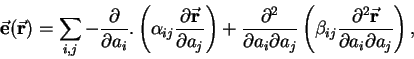
The term corresponding to the internal energies accumulated due to
elastical deformation
.
The term corresponding to the internal energies accumulated due to
elastical deformation
![]() is estimated from the following
empirical consideration:
is estimated from the following
empirical consideration:
By applying the weighted norms of equation (2), the following simplified deformation energy:
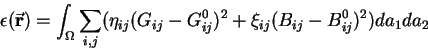
From equation (3)
an approximation for the
internal force
![]() is suggested:
is suggested:
Since quantities ![]() are related to surface stretching,
while the values for
are related to surface stretching,
while the values for ![]() are related
to curvature, the measures of deformation follow from these
quantities and the surface's behavior of resistance to external forces
will be as much effective as greater are the values assigned to the elasticity
parameters.
are related
to curvature, the measures of deformation follow from these
quantities and the surface's behavior of resistance to external forces
will be as much effective as greater are the values assigned to the elasticity
parameters.
Discretization
The discretization turns the partial differential equation of motion into a system of coupled ordinary differential equations.
The continuous space ![]() is discretized to a MxN-node mesh, where each
node
is discretized to a MxN-node mesh, where each
node ![]() represents a discrete point (or a nodal variable)
represents a discrete point (or a nodal variable)
![]() in 3D space. To the set of nodal variables
in 3D space. To the set of nodal variables
![]() defined for MN nodes we call function mesh and
we denote it
defined for MN nodes we call function mesh and
we denote it
![]() .
.
Equations (4) and (5)
are respectively discretized to
![\begin{displaymath}
e_{ij}[m,n]=\sum^{2}_{i,j}-D^{-}_{i}({\bf\vec p})[m,n]+D^{(-)}_{ij}({\bf\vec q})[m,n]
\end{displaymath}](img24.gif)
and
One can observe that the values for the difference operators are not
determined for points laying at the boundaries of domain ![]() .
Nevertheless, a natural condition of boundary can be simulated by
assigning a
.
Nevertheless, a natural condition of boundary can be simulated by
assigning a ![]() value to any difference operator of
equation (7)
that refers to points
value to any difference operator of
equation (7)
that refers to points
![]() not belonging to the set of points MN of the mesh.
not belonging to the set of points MN of the mesh.
If the nodal variables in function meshes ![]() and
and ![]() are grouped, respectively, into column matrices
are grouped, respectively, into column matrices ![]() e
e ![]() of dimension MN, then equation (6) can be
written in matrix form
of dimension MN, then equation (6) can be
written in matrix form
The discrete form of the equation of motion can then be expressed by
the following coupled system of differential equations:
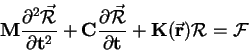
 is the diagonal matrix formed by the mass density of
each element,
is the diagonal matrix formed by the mass density of
each element,
 , the diagonal matrix formed by the dumping density of
each element and
, the diagonal matrix formed by the dumping density of
each element and
 , the column matrix containing the external force
applied to each element, calculated from
, the column matrix containing the external force
applied to each element, calculated from
 .
.
To simulate the dynamics of a non-rigid object, the system of differential equations (11) must be integrated through time. Those equations will be integrated using a step-by-step process, which now converts a system of non-linear differential equations into a sequence of linear systems.
The time interval from t=0 to t=T is subdivided into smaller time intervals of
same duration ![]() and the integration process carries out the
calculations for the sequence of approximated solutions for instants
t, t+
and the integration process carries out the
calculations for the sequence of approximated solutions for instants
t, t+![]() , t+2
, t+2![]() , ... , T. Computing
, ... , T. Computing
![]() in
in ![]() and
and ![]() in t, and substituting the
discrete-time approximations
in t, and substituting the
discrete-time approximations
in equation (11) it is obtained
where
and
The column matrix of speed ![]() is given by:
is given by:
| (17) |