Demo Script
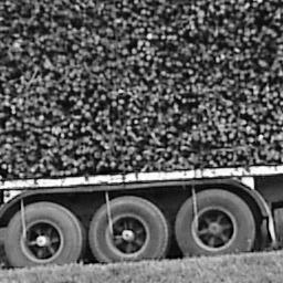
Image read and histograming

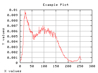
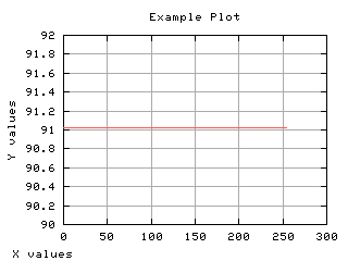
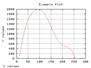
Normalized histogram
If the histogram is divided by the number of pixels in the image, it can be seen as a probability distribution. The sum of each values gives one. The mean gray level can be computed from the normalized histogram.
>>> import MLab
>>> h = 1.*H/Numeric.product(f.shape)
>>> print Numeric.sum(h)
1.0
>>> mt = Numeric.sum(x * h)
>>> st2 = Numeric.sum((x-mt)**2 * h)
>>> if abs(mt - MLab.mean(Numeric.ravel(f))) > 0.01: iaerror('error in computing mean')
error in computing mean
>>> if abs(st2 - MLab.std(Numeric.ravel(f))**2) > 0.0001: iaerror('error in computing var')
error in computing var
>>> print 'mean is %2.2f, var2 is %2.2f' % (mt, st2)
mean is 91.03, var2 is 2873.86
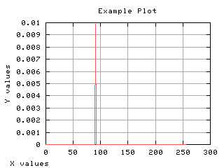
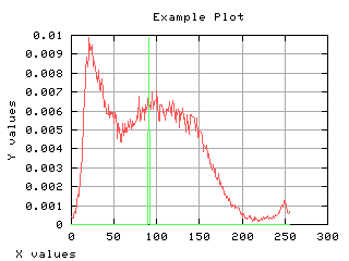
>>> maux = 0 * h
>>> maux[int(mt)] = max(h)
>>> g,d1 = iaplot(x,h)
>>> g,d2 = iaplot(x,maux)
>>> g.plot(d1, d2)
>>>
 |
 |
|
| x,h | x,maux |
 |
|
| d1, d2 |
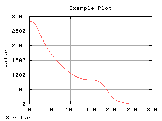
Two classes
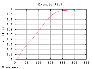
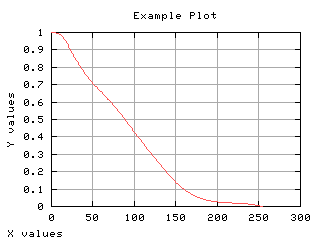
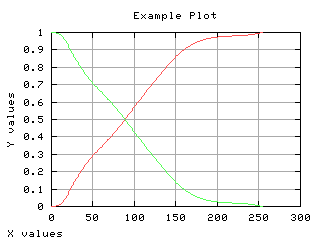
Suppose the pixels are categorized in two classes: smaller or equal than the gray scale t and larger than t. The probability of the first class occurrence is the cummulative normalized histogram. The other class is the complementary class.
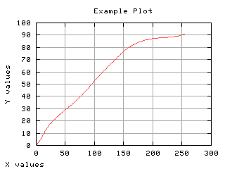
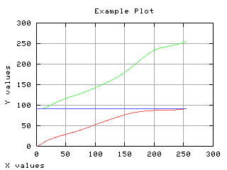
Mean gray level of each class
The mean gray level as a function of the thresholding t is computed and displayed below.
>>> m0 = MLab.cumsum(k * h[0:-1]) / (1.*w0)
>>> m1 = (mt - m0*w0)/w1
>>> aux = (k+1) * h[1::]
>>> m1x = MLab.cumsum(aux[::-1])[::-1] / (1.*w1)
>>> mm = w0 * m0 + w1 * m1
>>> if max(abs(m1-m1x)) > 0.0001: iaerror('error in computing m1')
>>> g,d1 = iaplot(k,m0)
>>> g,d2 = iaplot(k,m1)
>>> g,d3 = iaplot(k,mm)
>>> g.plot(d1,d2,d3)
>>>
 |
 |
|
| k,m0 | k,m1 |
 |
 |
|
| k,mm | d1,d2,d3 |
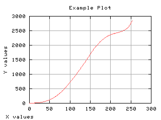
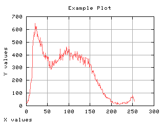
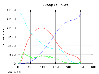
Variance of each class
The gray level variance as a function of the thresholding t is computed and displayed below.

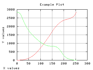
Class separability
The variance between class is a good measure of class separability. As higher this variance, the better the class clustering.
>>> sB2 = w0 * ((m0 - mt)**2) + w1 * ((m1 - mt)**2)
>>> sBaux2 = w0 * w1 * ((m0 - m1)**2)
>>> if max(sB2-sBaux2) > 0.0001: iaerror('error in computing sB')
>>> v = max(sB2)
>>> t = (sB2.tolist()).index(v)
>>> eta = 1.*sBaux2[t]/st2
>>> print 'Optimum threshold at %f quality factor %f' % (t, eta)
Optimum threshold at 93.000000 quality factor 0.694320
>>> g,d1 = iaplot(k, sB2)
>>> g,d2 = iaplot(k, H[0:-1])
>>> g,d3 = iaplot(k, s02)
>>> g,d4 = iaplot(k, s12)
>>> g.plot(d1, d2, d3, d4)
>>>
 |
 |
|
| k, sB2 | k, H[0:-1] |
 |
 |
|
| k, s02 | k, s12 |
 |
|
| d1, d2, d3, d4 |
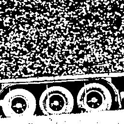
Thresholding
The thresholded image is displayed to illustrate the result of the binarization using the Otsu method.
>>> x_ = iashow(f > t)
(256, 256) Min= 0 Max= 1 Mean=0.472 Std=0.50
 |
|
| f > t |