iadftdecompose
Illustrate the decomposition of the image in primitive 2-D waves.

>>> import Numeric

>>> f = Numeric.ones((128, 128)) * 50

>>> x, y = [], map(lambda k:k%128, range(-32,32))

>>> for i in range(128): x = x + (len(y) * [i])

>>> y = 128 * y

>>> Numeric.put(f, iasub2ind([128,128], x, y), 200)

>>> iashow(f)

(128, 128) Min= 50 Max= 200 Mean=125.000 Std=75.00

>>> F = iadft(f)

>>> E = iadftview(F)

>>> iashow(E)

(128, 128) Min= 0 Max= 255 Mean=0.737 Std=11.72

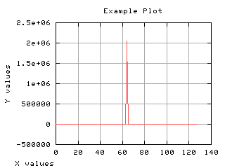
>>> g,d = iaplot(iafftshift(F[:,0]).real)

>>> g('set data style impulses')

>>> g.plot(d)

>>>