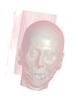
3D Medical Data Visualization Toolkit offer numerous visualization methods within a comprehensive visualization system, providing a flexible tool for surgeons and health professionals as well
as the visualization developer and researcher.
Our system offers the possibility to visualize 3D medical images from various devices,
Computed Tomography, Magnetic Resonance Imaging and others.
Basedon direct volume rendering with textures and ray casting, offers high image resolution,
provides interactive navigation within the volume through the movement of coronal,
sagittal and axial planes, with direct applications to medical diagnosis.
Tis project was performed as part of the requirementof the Course: 3D Visualization – IA369, lectured by Wu Shin Ting, at School of Electrical and Computer Engineering, State University of Campinas.
In a nutshell, the
Direct Volume Rendering, hereafter DVR, maps the 3D
scalar field to physics quantities (color and opacidade) that describe light interactions at the
respective point in the 3D space. The visualizations can be created without creating intermediate geometric structure, such as polygons comprising an isosurface, but simply by a “direct” mapping from volume data points to composited image elements.
Formally, a DVR can be described as function that visually extracts
information from 3D scalar field:

ie, a function from 3D space to a
single-scalar value.
1.1. SCALAR DATA VOLUME.
Scalar data volume (3D data set) can come from a variety of different areas of applications. Currently,
the images acquired by medical diagnostic processes are the main 3D data
generated. This medical imaging is performed by CT (Computerized Tomography), RMI (Resonance Magnetic Imaging),
Nuclear Medicine and Ultrasound.}
All this medical imagingmodalities have in common that a discretized volume
data set is reconstructed from the detected feedback (mostly, radiation).
In addition to thesesources, simulations also generate
data sources for volume rendering, ie computational
fluid dynamics simulations and simulations of fire and explosions for especial effects. I don’t forgot said that the voxelization also generate data sets.
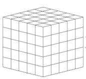
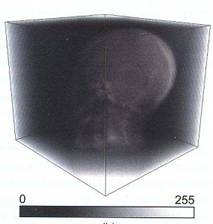
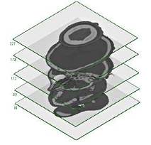
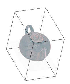
The next figure shows anexample of volume data set:
Figure 1. (Left) Volume data set given a discrete
uniform grid. (Right) Final volume rendition with its Transfer
Function
In a regular volumetric grid, each volume element is called voxel (Volume Element), that’s represent a
single value that is obtained by sampling the immediate area surrounding the voxels.
1.2. COMPOSITION.
All DRV algorithms perform same core composition
scheme: either, front-to-back composition
or back-to-front composition. Basically, the difference is where the origin of the
ray traversal.
1.3. ALGORITHMS FOR DIRECT VOLUME RENDERING.
Volume rendering techniques can be classified as either object-order or image-order methods. The object-order methods scan the 3D volume in
its objects space, then project it onto the image
plane. The other strategy, use the 2D image space (image plane) as the starting
point for volume traversal.
In the project, we implemented Texture Slicing and Ray
Casting algorithms, for object-order and image-order techniques,
respectively.
Until a few years ago, texture slicing was the dominant method for GPU (Graphic Process Unit) based volume rendering. In this
algorithm: 2D slices located in 3D object space are used to sample the volume. The
slices are projected onto the image plane and combined according of composition
scheme. Slices ordered either in a
front-to-back or back-to-front fashion and the composition equations has to be chosen
accordingly.
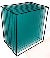
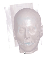
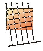
Figure 2.
Object Order Approach (Left) Sampling data set.
(Right) Slices textured obtained.
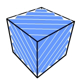
Figure 3.
Object Order Approach (Left) Proxy geometry – polygonal slices. (Right) Final volume rendering.
The main advantage of this method is that it is directly supported by
graphics hardware because it just needs texture support and blending (composition
scheme). One drawback is the restrictions to uniform grids.
The basic component on texture
slicing is built upon:
-
Geometry Set-Up. In this stage we perform the
decomposition of the volume data set into polygonal slices. It calculate the position and texture coordinates in 3D of the
vertices that need to be rendered.
-
Texture Mapping. This component determines how the
volume data is stored in memory and how the data is used during fragment
processing. In the current project we used Texture 3D supported in all actually
graphics cards.
-
Composition Set-Up. This components defines how the
color values of the draw textured polygons are successively combined to create the
final rendition.
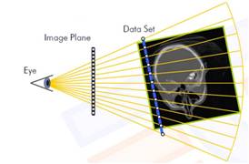
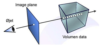
Ray casting is the most popular image-order method for volume rendering.
In this algorithm we composite along rays that are traversed form the camera. For each pixel in the image, a single ray cast into the volume, then the
volume data is resampled at discrete positions along
the ray. The natural traversal order is front-to-back because the rays are
started at the camera, but also the way the ray traversal can be adversely.
Figure 4.Image Order Approach: Ray Casting.
At final rendering only 0.2% to 4% of all fragments are visible, then
ray casting in an appropriate approach to address these issues. Because the
rays are handled independently from each other, ray casting allows several
optimizations:
Moreover, ray casting is very good for uniform grids and tetrahedral
grids.
Pseudo code of ray casting:
|
Determine volume entry position
Compute ray direction
While (ray position into volume)
Access data value a current position
Composition of color y opacidade (apply
transfer function)
Advance position along ray
End While
|
The main objective of volume rendering is extract information over thesescalar values in the 3D grid, identifying features of interest. In DVR the central ingredient is the assignment of optical properties (color and opacidade) to the values comprising the volume dataset. This is the role of the transfer function.
As simple and direct as that mapping is, it is also extremely fexible, because of the immense variety of possible transfer functions. However, that flexibility becomes a weakness because of the difficulty to se appropriately the the most important parameter for producing
a meaningful and intelligible volume rendering
In the simplest type of transfer function, the domain is the scalar data value and the range is color and opacity, by example, a 1D transfer function maps one RGBA value for every isovalue [0, 255] of scalar data set.
Transfer functions can also be generalized by increasing the dimension of the function’s domain. These can be termed multidimensional transfer functions. In scalar volume datasets, a useful second dimension is that of gradient magnitude.
Formally,
a transfer function could be describe as:

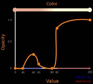
The next figure show a simple 1D transfer function based on linear ramps between user-specifed control points.
Figure 5.1D Transfer Function.
From: http://graphicsrunner.blogspot.com/2009/01/volume-rendering-102-transfer-functions.html
The process of finding an appropriate transfer function is
often referred to as classifications. The design of a transfer function in general is a manual, tedious an time- consuming procedure, that requires detailed
knowledge of the special structures that are represented by the data set.
Our 3D Medica Data Visualization Tool is on the two algorithms most widely used in direct volume rendering. We implemented 3D Textured slicing and Single Pass Ray Casting based on GPU.
-
Hardware Used
-
Intel
computer, CPU Core 2 Duo 3.0 GHz , 03 GB RAM, with graphic card NVIDIA GeForce
GT-240 (CUDA 96 CORES, 512 MB internal memory).
-
Operating System: Ubuntu Linux 10.
We recommend update drivers and libraries extensions with lasts versions.
Texture 3D have several advantages over 2D
texture-based volume rendering, caused by the fixed number of slices and its
statics alignment within the object’s coordinates system.
Despitethe use of 3D textures, we need decomposing the volume object into planar
polygons: 3D textures do not represent volumetric rendering primitives.
3D textures allow the slice polygons to be positioned arbitrarily in the 3D space
according the viewing directions: is an viewport – aligned slices as
displayed in the next figure.
Figure 6.View aligned slices. Decomposition of the volume object into viewport-aligned polygon slices.
3.1.1. Geometry Set-Up
The procedure of intersections calculations between the bounding box and the stack of viewport-aligned slices is computationally more complex. Moreover, these polygonal slices must be recomputed whenever the viewing directions changes.
One method for computing the plane-box-intersection can be formulate as a sequence of three steps:
-
Compute the intersections points between the slicing plane and the straight lines that represent the edges of the bounding box.
-
Eliminate duplicate and invalid intersections points.
-
Sort the remaining intersection points to form a closed polygon.
We perform the plane-box- intersectioncalculation on the CPU and the resulting polygons slices are uploaded to GPU.
3.1.2. Compute the Plane-Box-Intersection
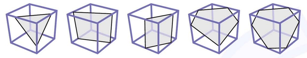
Compute the intersection between a cube and an arbitrary oriented plane is a complicated task. For complicate matter
further, these intersections points results in a polygon with three to six
vertices; these are illustrated in next figure.
Figure 7.Polygons resulting form intersections plane-box. Polygon has between three and six vertices.
To
facilitate the calculations, we use a plane in Hessian normal form:

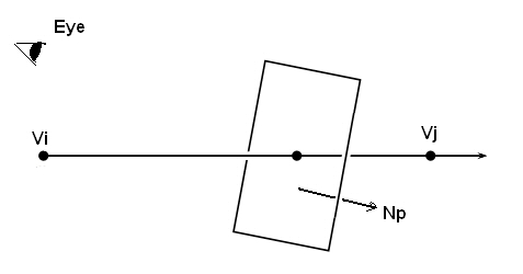
Where Np denotes the normal
vector of the plane and d is the distance to the origin.
Then the problem is
reduced to compute the intersection of a plane with an edge (the edge -ray formed by
two vertices Vi and Vj of the
volume bounding box).
Figure 8. Ray - Plane - Intersection
For resolving this case, we used the algorithm for Ray-Plane Intersection for all edges of the bounding box, based on the equation of the line:
With
Solved for
The denominator becomes zero only if the edge is
coplanar with the plane, in this case, ignore the intersection. We have a valid
intersection only
A detailed description of Ray – Plane- Intersection Algorithm you can
find in 3D Computer Graphics: a mathematical introduction with OpenGL book of Samuel R.Buss.
3.1.3. Implementatios details
We probe worked two alternatives, first, manipulating the OpenGL Texture
Matrix; second, applying transformations to move the camera around
the object.
- Manipulating Texture Matrix:
- In this case, the Eye direction is fexed to (0.0, 0.0,-1.0) and compute the intersections over the boundig box vertices (world coordinates) transformed with the Texture Matrix.
|
void planeBoxInit() {
int i;
for(i=0;
i<NUMPLANES; i++){
slicingPlane[i][X] = 0;
slicingPlane[i][Y] = 0;
slicingPlane[i][Z] = (-3.5f*i)/NUMPLANES
+ 1.75f;
}
np[X] = 0; np[Y] = 0; np[Z] = -1; //normal vector
v[0][X] = -1; v[0][Y] = 1; v[0][Z] = 1;
//bounding box vertices
v[1][X]
= 1; v[1][Y] = 1; v[1][Z] = 1;
v[2][X] = -1; v[2][Y] = -1; v[2][Z]
= 1;
v[3][X] = -1; v[3][Y] = 1; v[3][Z] = -1;
v[4][X] = 1; v[4][Y] = 1; v[4][Z] = -1;
v[5][X] = 1; v[5][Y] = -1; v[5][Z] = 1;
v[6][X] = -1; v[6][Y] = -1; v[6][Z] =
-1;
v[7][X]
= 1; v[7][Y] = -1; v[7][Z] = -1;
e[0].i
= &v[0]; e[0].j = &v[1]; //twelve edges
e[1].i = &v[0]; e[1].j = &v[2];
e[2].i
= &v[0]; e[2].j = &v[3];
e[3].i
= &v[1]; e[3].j = &v[4];
e[4].i
= &v[2]; e[4].j = &v[5];
e[5].i
= &v[3]; e[5].j = &v[6];
e[6].i
= &v[4]; e[6].j = &v[7];
e[7].i
= &v[5]; e[7].j = &v[7];
e[8].i
= &v[6]; e[8].j = &v[7];
e[9].i
= &v[1]; e[9].j = &v[5];
e[10].i
= &v[2]; e[10].j = &v[6];
e[11].i
= &v[3]; e[11].j = &v[4];
}
|
|
void detectPlaneBoxIntersections(int
*nIntersects, vertex3D intersectCoords[NUMPLANES][6]) {
int i, j, k, l;
float lambda, denom, menorDist;
edge3D
edgeIJ;
for(i=0;
i<NUMPLANES; i++){
nIntersects[i]
= 0;/ plano
[i]
for(j=0; j<12; j++){// 12 edges
edgeIJ[X]
= e[j].j[0][X] - e[j].i[0][X];
edgeIJ[Y] = e[j].j[0][Y] - e[j].i[0][Y];
edgeIJ[Z]
= e[j].j[0][Z] - e[j].i[0][Z];
denom = dotProduct(np, edgeIJ);
if (denom != 0){//
lambda = (-dotProduct(np, slicingPlane[i]) - dotProduct(np, e[j].i[0]))
/ denom;
if(lambda >= 0 && lambda <= 1){
intersectCoords[i][nIntersects[i]][X]
= lambda*edgeIJ[X] + e[j].i[0][X];
intersectCoords[i][nIntersects[i]][Y]
= lambda*edgeIJ[Y] + e[j].i[0][Y];
intersectCoords[i][nIntersects[i]][Z]
= lambda*edgeIJ[Z] + e[j].i[0][Z];
nIntersects[i]++;
}
}
}
|
|
void displayPLANEBOX() {
.......//more code
//bounding Box transformations
glPushMatrix();
glRotatef(yrot,
0, Y_AXIS, 0);
glRotatef(xrot,
X_AXIS, 0, 0);
glTranslatef(xtrans,
ytrans, ztrans);
glGetFloatv(GL_TEXTURE_MATRIX,
(GLfloat *) modeltexture);
glPopMatrix();
//Matrix
Texture transformations
glTranslatef(xtransini,
ytransini, ztransini);
glRotatef(-xrot,
X_AXIS, 0, 0);
glRotatef(-yrot,
0, Y_AXIS, 0);
glTranslatef(-xtransini,
-ytransini, -ztransini);
glTranslatef(-xtrans,
-ytrans, -ztrans);
planeBoxInit();
multVerticesModelview();
detectPlaneBoxIntersections(numIntersections,
intersectionCoords);
.......//more code
}
|
- Moving camera around the object
- We use spherical coordinates for rotate the camera around a fixed cube position. Basically, modifiy the Eye and Up vectors.
- In this approximation, the new eye direction is the Normal of Hessian Plane, then compute the intersection of Plane-Box with twelve edges for N (number) planes especified.
|
//Camera
position
typedef struct {
//Position of
camera
Vector3 Eye;
Vector3
Center;
Vector3 Up;
} Camera;
|
- Spherical
to Cartesian conversion
|
//more code
cam.Eye.x = radio * sin(theta *
0.0174532) * sin(phi * 0.0174532);
cam.Eye.y = radio * cos(theta *
0.0174532);
cam.Eye.z = radio * sin(theta * 0.0174532)
* cos(phi * 0.0174532);
//more code
|
- The N (number) of planes determines the resolution
of volume rendered (ie, 256 planes).
.
3.1.4 Example 3D Texture Slicing
- Loading data set as 3D Texture:
|
glBindTexture(GL_TEXTURE_3D,
tex3Dvolume);
glTexParameteri(GL_TEXTURE_3D,
GL_TEXTURE_MIN_FILTER, GL_LINEAR);
// when this
texture needs to be magnified to fit on a big polygon, use linear
interpolation of the texels to determine the color
glTexParameteri(GL_TEXTURE_3D,
GL_TEXTURE_MAG_FILTER, GL_LINEAR);
// we want
the texture to repeat over the S axis, so if we specify coordinates out of
range we still get textured.
glTexParameteri(GL_TEXTURE_3D,
GL_TEXTURE_WRAP_S, GL_CLAMP);
glTexParameteri(GL_TEXTURE_3D,
GL_TEXTURE_WRAP_T, GL_CLAMP);
glTexParameteri(GL_TEXTURE_3D,
GL_TEXTURE_WRAP_R, GL_CLAMP);
// this is a
3d texture, GL should store it in RGBA
glTexImage3D(GL_TEXTURE_3D, 0, GL_RGBA,
XDIM, YDIM, ZDIM, 0, GL_LUMINANCE, GL_UNSIGNED_BYTE, voxels);
|
- Important: at the beginning of the program, you must set the uniform variables of fragment program
|
..........
//Setting
shader's uniform variables
GLint vol =
glGetUniformLocation(programObject, "VOLUME");
GLint tf =
glGetUniformLocation(programObject, "TRANSFERFUNCTION");
glUseProgram(programObject);
// Use The Program Object Instead Of Fixed Function OpenGL
printProgramInfoLog(programObject);
//Information log
//
Set the uniform variables values
glUniform1i(vol, 0);
glUniform1i(tf, 1);
.......
|
- Then, you must set the textures
|
//Activate and select 3D Texture
glActiveTexture(GL_TEXTURE0);
glBindTexture(GL_TEXTURE_3D,
tex3Dvolume);
glEnable(GL_TEXTURE_3D);
//Activate
and select 1D Texture glActiveTexture(GL_TEXTURE1);
glBindTexture(GL_TEXTURE_1D, tex1Dtf); glEnable(GL_TEXTURE_1D);
|
The escalar value is used as an index into a post-interpolative transfer function
|
uniform sampler3D VOLUME;
uniform sampler1D TRANSFERFUNCTION;
void main(void){
float position ;
vec4 color;
position = texture3D(VOLUME,
gl_TexCoord[0].xyz).r;
//get volume data
gl_FragColor =texture1D(TRANSFERFUNCTION, position);}
}
|
Figure 8. Volume Rendering without illumination, 768 slices with a simple 1D Transfer Function
-
A Central Difference method can be use for compute on CPU (pre-processing step) the gradient vector (x,y,z) of scalar field. Afther normalized this vector to [-1,1], it is scaled to [0,1] for send to GPU.
-
We combine the scalar field into a single RGBA texture. In RGB is stored the gradient vector and in A the scalar value. The escalar value is used as an index into a post-interpolative transfer function.
-
Setting the light and material properties:
|
void setLight(void)
{
GLfloat globalAmbient[] = { 0.2f, 0.2f,
0.2f, 1.0f };
GLfloat ambient[] = { 0.2f, 0.2f, 0.2f,
1.0f };
GLfloat diffuse[] = { 0.4f, 0.5f, 0.4f,
1.0f };
GLfloat specular[] = { 0.4f, 0.4f,
0.4f, 1.0f };
GLfloat position[] = { 0.0f, 0.0f,
1.0f, 1.0f };
glLightfv(GL_LIGHT0, GL_AMBIENT,
ambient);
glLightfv(GL_LIGHT0, GL_DIFFUSE,
diffuse);
glLightfv(GL_LIGHT0, GL_SPECULAR,
specular);
glLightfv(GL_LIGHT0, GL_POSITION,
position);
glLightModelfv(GL_LIGHT_MODEL_AMBIENT,
globalAmbient);
glEnable(GL_LIGHTING);
glEnable(GL_LIGHT0);
glEnable(GL_NORMALIZE);
}
void setMaterial(void)
{
// Material
parameters:
GLfloat material_Ka[] = { 0.2f, 0.2f,
0.2f, 1.0f };
GLfloat material_Kd[] = { 0.4f, 0.4f,
0.4f, 1.0f };
GLfloat material_Ks[] = { 0.4f, 0.4f,
0.4f, 1.0f };
GLfloat material_Ke[] = { 0.0f, 0.0f,
0.0f, 0.0f };
GLfloat material_Se = 70.0f;
glMaterialfv(GL_FRONT_AND_BACK,
GL_AMBIENT, material_Ka);
glMaterialfv(GL_FRONT_AND_BACK,
GL_DIFFUSE, material_Kd);
glMaterialfv(GL_FRONT_AND_BACK,
GL_SPECULAR, material_Ks);
glMaterialfv(GL_FRONT_AND_BACK,
GL_EMISSION, material_Ke);
glMaterialf(GL_FRONT_AND_BACK,
GL_SHININESS, material_Se);
}
|
|
vec4 shading
(vec3 N, vec3 V, vec3 L){
vec4
ambient;
vec4
diffuse;
vec4
specular;
vec3 H = normalize(L+V); //calculate
halfway vector
//calculate Ambient Term
//ambient =
gl_FrontLightProduct[0].ambient;
ambient =
gl_FrontLightProduct[0].ambient;
//calculate Diffuse Term
float diffuseLight = max(dot(L,N),0.0);
diffuse =
gl_FrontLightProduct[0].diffuse * diffuseLight ;
//calculate Specular Term
float specularLight =
pow(max(dot(H,N),0.0), gl_FrontMaterial.shininess);
if(diffuseLight<=0.0) {
specularLight = 0.0;
}
specular =
gl_FrontLightProduct[0].specular * specularLight ;
return ambient+ diffuse + specular;
}
|
|
uniform
sampler3D VOLUME;
uniform
sampler1D TRANSFERFUNCTION;
void
main(void){
vec4 color;
mat4 mvi = gl_ModelViewMatrixInverse; //matrix
model-view-inverse
//Compute the camera position by
translating the origin to the center
//of
the volume
vec4
camera = mvi[3];
vec4 sample =texture3D(VOLUME,
gl_TexCoord[0].xyz); //sample
//expand and normalize the normal
vector
vec3 N =
normalize(2.0*sample.xyz-vec3(1.0,1.0,1.0));
//because datas were in [-1,1]
//light direction
vec3 L =
normalize(gl_TexCoord[0].xyz - (vec3(
gl_LightSource[0].position * gl_ModelViewMatrix)));
//view direction
vec3 V =
normalize(gl_TexCoord[0].xyz - camera.xyz);
//applying
transfer function
color =texture1D(TRANSFERFUNCTION, sample.w);
color.rgb
+= shading(N,V,L).rgb;
gl_FragColor = color;
}
|
Figure 9. Volume Rendering with Blinn Phong illumination, 798 slices with pre-computed-gradient and 1D Transfer Function
- The advent of powerful GPU fragment shader hardware now allows us to compute gradient on the fly during rendering, whereever they are needed.
- Fragment program for on-the-fly gradient stimation.
#define DELTA (0.001)
#define THRESHOLD (0.01)
uniform sampler3D VOLUME; //component r=g=b= scalar value a=1
uniform sampler1D TRANSFERFUNCTION; //rgba = assing cor
vec4 shading (vec3 N, vec3 V, vec3 L); //shading function
//float position ;
//vec4 color;
//position = texture3D(VOLUME, gl_TexCoord[0].xyz).r; //get volume data
//gl_FragColor =texture1D(TRANSFERFUNCTION, position);
void main(void){
vec3 position = gl_TexCoord[0].xyz; //space position of one scalar sample
mat4 mvi = gl_ModelViewMatrixInverse; //matrix model-view-inverse
//Compute the camera position by translating the origin to the center
//of the volume
vec4 camera = mvi[3]; //camera position
//vec3 camera = gl_ModelViewMatrixInverse[3].xyz; //camera world position
//texture sample for the scalar value
float sample =texture3D(VOLUME, position.xyz).r;
//applying transfer function
vec4 color =texture1D(TRANSFERFUNCTION, sample); //rgba
if (color.a>THRESHOLD){
vec3 sample1, sample2;
//calculate six texture samples for the gradient
sample1.x = texture3D(VOLUME, (position.xyz - vec3(DELTA, 0.0, 0.0))).x;
sample2.x = texture3D(VOLUME, (position.xyz + vec3(DELTA, 0.0, 0.0))).x;
sample1.y = texture3D(VOLUME, (position.xyz - vec3(0.0, DELTA, 0.0))).x;
sample2.y = texture3D(VOLUME, (position.xyz + vec3(0.0, DELTA, 0.0))).x;
sample1.z = texture3D(VOLUME, (position.xyz - vec3(0.0, 0.0, DELTA))).x;
sample2.z = texture3D(VOLUME, (position.xyz + +vec3(0.0, 0.0, DELTA))).x;
//calculate the central difference and normalization
vec3 N = normalize(sample2-sample1);
//calculate light direction
//vec3 L = normalize( gl_TexCoord[0].xyz - (gl_ModelViewMatrixInverse * gl_LightSource[0].position).xyz);
vec3 L = normalize(position.xyz - (vec3( gl_LightSource[0].position *gl_ModelViewMatrix))); //positional light
//calculate view direction
vec3 V = normalize(position.xyz - camera.xyz);
//compute final color
color.rgb += shading(N,V,L).rgb;
}
gl_FragColor = color;
}
|
- The Shading function is the same used in the previous section.
Figure 10. Blinn Phong illumination, 798 slices with on-the-fly gradient stimation
|
#define STEPSIZE (0.005)
uniform sampler3D VOLUME;
uniform sampler1D TRANSFERFUNCTION;
uniform vec4 camDir;
void main(void){
vec3 volExtentMin = vec3(0.0, 0.0, 0.0);//mim value of boundingbox
vec3 volExtentMax = vec3(1.0, 1.0, 1.0);//max value of boundingbox
vec4 color = vec4(0.0 , 0.0 , 0.0 , 0.0); //initialize to zero the final color
//vec4 camera = gl_ModelViewMatrixInverse[3]; //Compute the camera world position as matrix model-view-inverse
//vec4 camDir = vec4(0.0, 0.0,-1.0,0.0); //camera direction for paralell projection
//RAY CASTING ALGORITHM
//(1)determine volume entry position
vec3 position = gl_TexCoord[0].xyz;
//(2)compute ray direction
vec3 direction = normalize((gl_ModelViewMatrixInverse*camDir).xyz);
//direction.z = -direction.z; //When mapped textured to [-1,1] in view order (without inversing coodinates)
//(3) ray traversal loop
for(int i=0; i<250;i++){
//(3.1) access data value at current position
float scalar =texture3D(VOLUME, position).r; //scalar value
//(3.2) apply transfer function
vec4 src = texture1D(TRANSFERFUNCTION, scalar);
src *= src.a; //Compute associated color of voxel
//Make the values in visible range
src = clamp (src, 0.0, 1.0);
//(3.3) front-to-back composition
color += (1.0 - color.a)*src;
color.a += src.a;
//(3.4) advance ray position along ray direction
position += direction*STEPSIZE;
//(3.5) ray termination test
vec3 temp1 = sign(position-volExtentMin);
vec3 temp2 = sign(volExtentMax-position);
float inside = dot(temp1, temp2);
//is not in the volume, exit
// terminate if opacity > 1 or the ray is outside the volume
if (inside<3.0 || color.a >0.99)
break;
}
gl_FragColor= color;
}
|
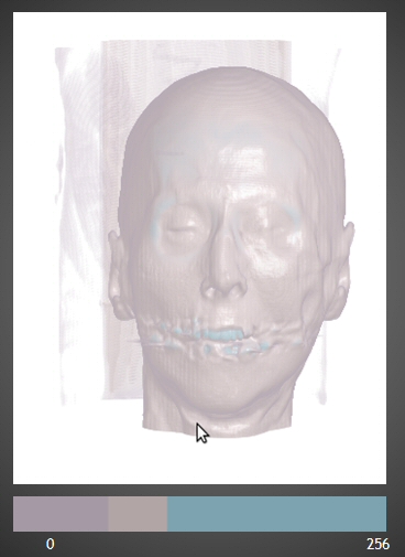
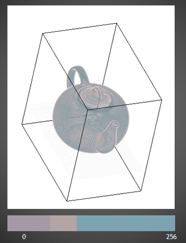
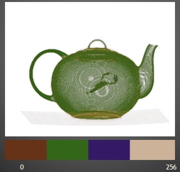
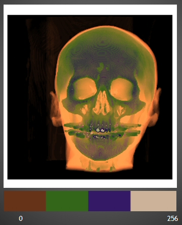
Figure 11. Data set redered with ray casting algorith and 1D Transfer Function
Figure 12. Data set redered with ray casting algorith and 1D Transfer Function
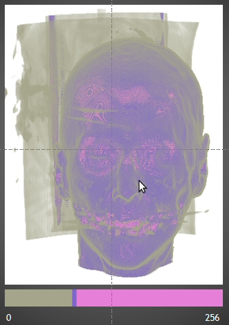
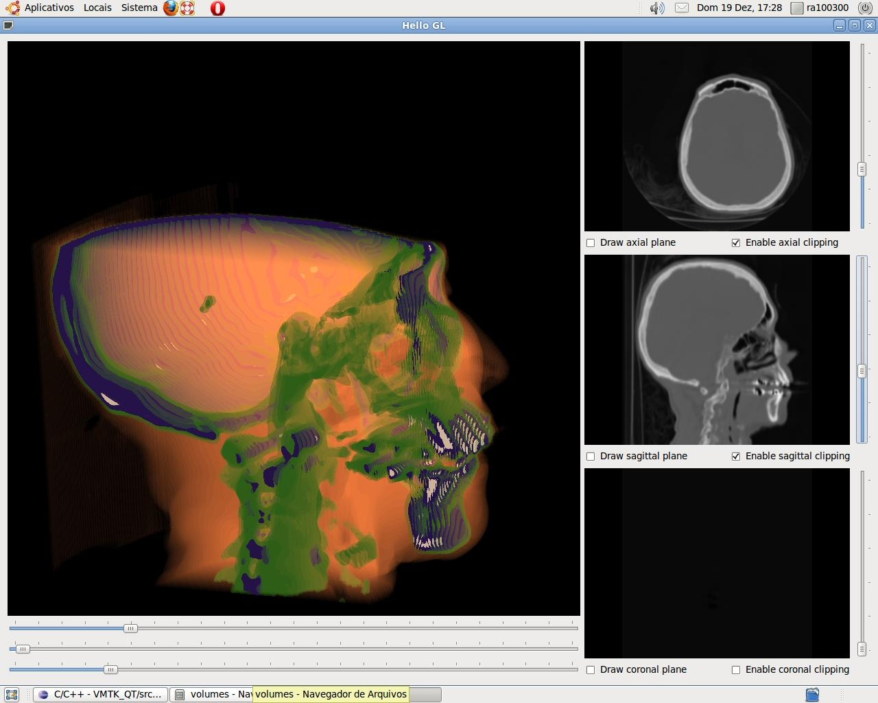
-
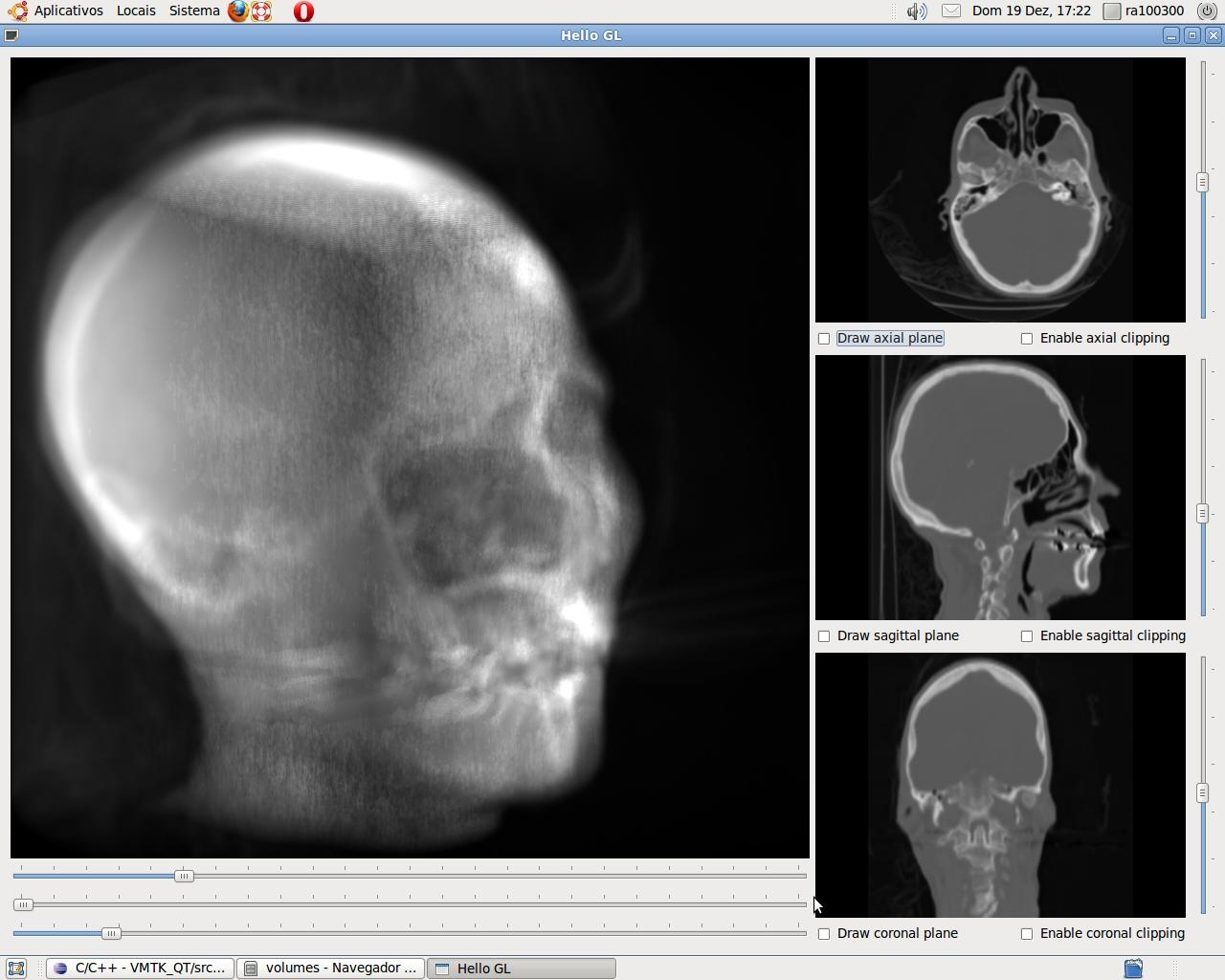
Using QT Framework, we develop and implement the first prototype of the 3D Medical Data Visualization based on on ray casting algorithm.
-
This offers interactive cut and visualization of coronal,
sagittal and axial planes.
-
Next, we present
some screenshots
Figure 13. screenshot of 3D Medical Data Visualization
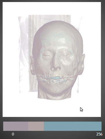
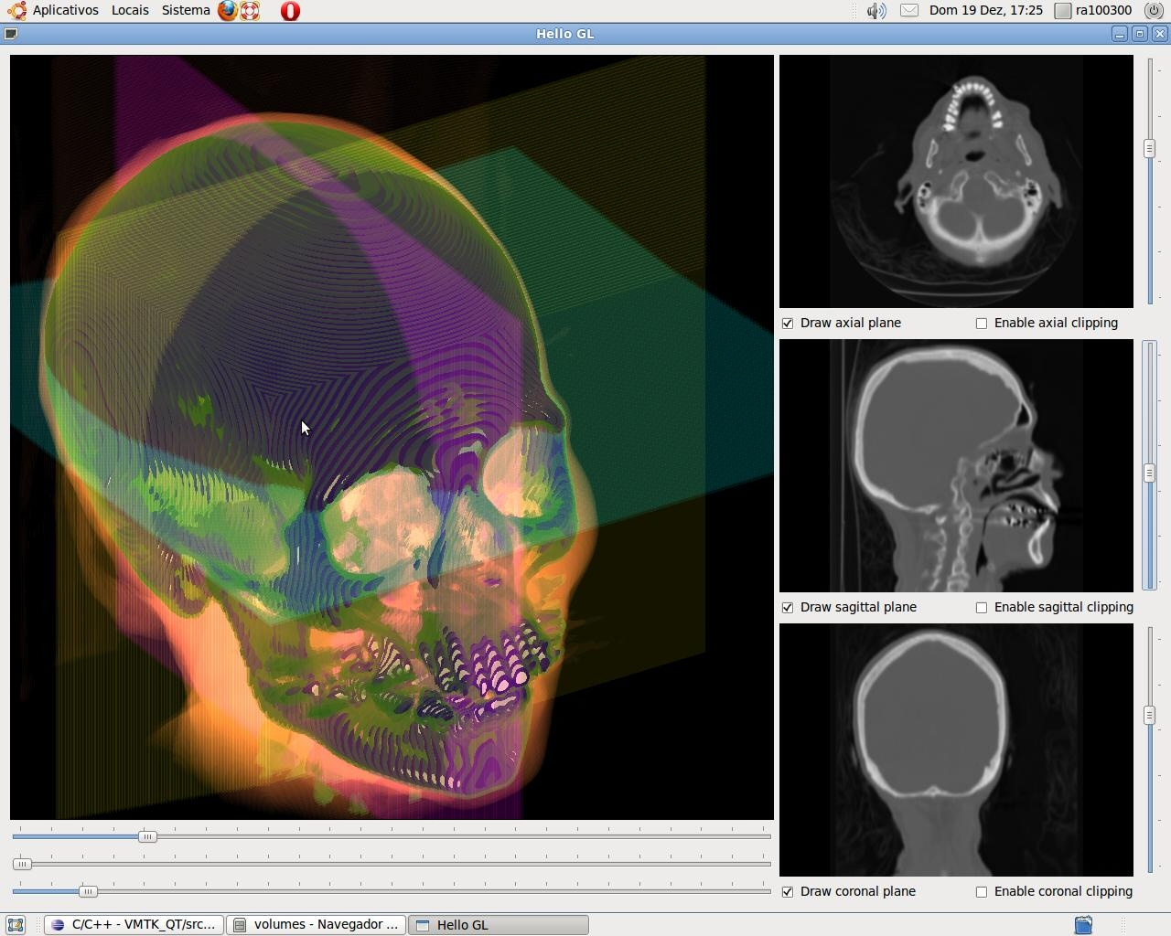
Figure 14. screenshot of 3D Medical Data Visualization
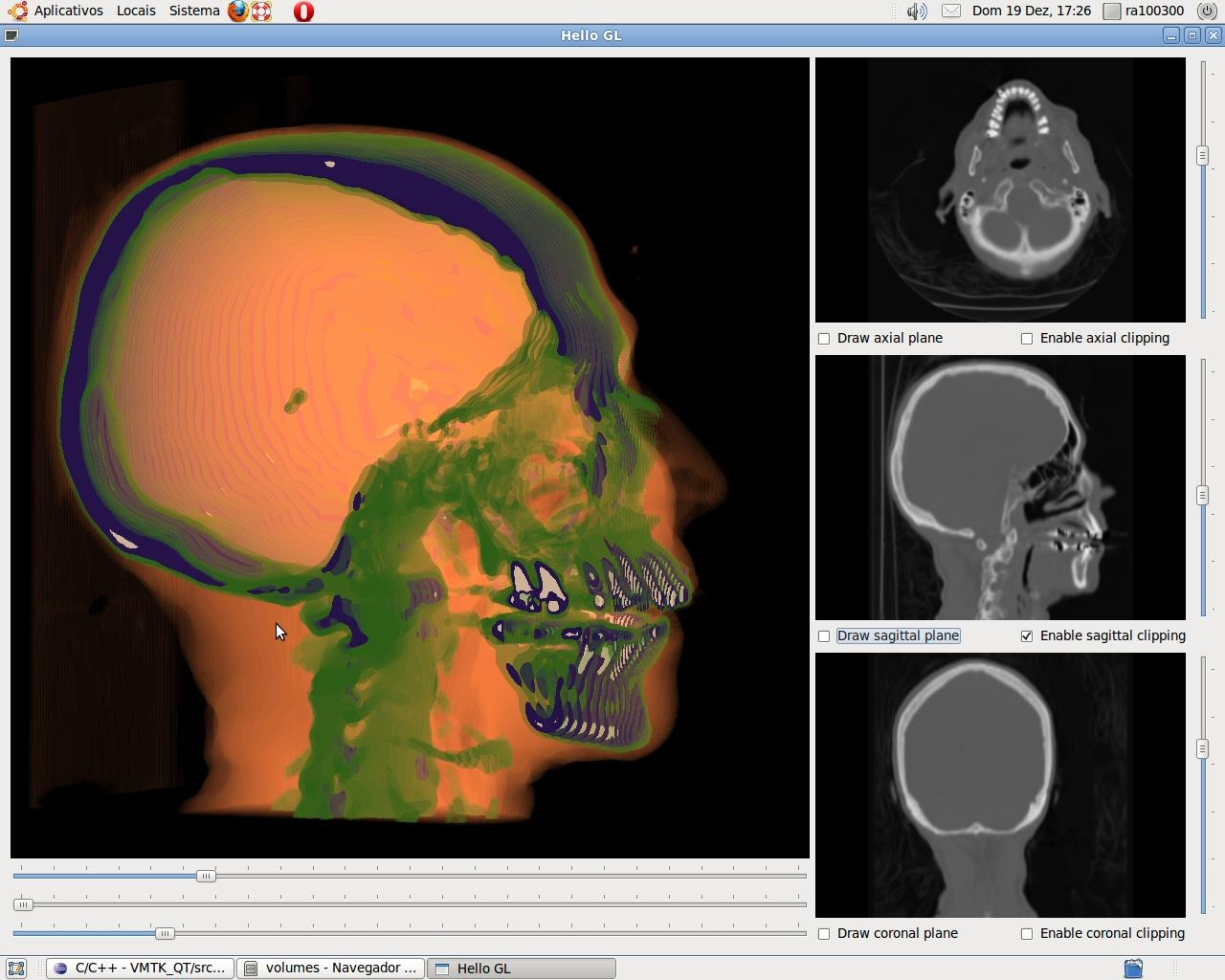
Figure 15. screenshot of 3D Medical Data Visualization
Figure 16. screenshot of 3D Medical Data Visualization